-
import numpy as np
import pandas as pd
Create Object
Series Data 형성
obj = pd.Series([1,3,5,np.nan,6,8])

obj =>
0    1.0
1    3.0
2    5.0
3    NaN
4    6.0
5    8.0
dtype: float64
DataFrame Data 형성
import pandas as pd
import numpy as np

dates = pd.date_range('20200902', periods=6)

dates=>
DatetimeIndex(['2020-09-02', '2020-09-03', '2020-09-04', '2020-09-05',
               '2020-09-06', '2020-09-07'],
              dtype='datetime64[ns]', freq='D')

df = pd.DataFrame(np.random.randn(6,4), index=dates, columns=list('ABCD'))

df=>
                   A         B         C         D
2020-09-02  0.676201 -0.735438  0.312747 -1.843620
2020-09-03 -0.358015  1.128569  0.738395  0.170064
2020-09-04 -1.307082 -0.417756  0.165525 -1.152548
2020-09-05  0.210957 -1.450819 -1.006740  1.197188
2020-09-06  0.554652 -1.910535 -1.145034 -0.563270
2020-09-07 -0.417373  2.479437 -1.287300 -1.128281


df2 = pd.DataFrame({'A':1.,
                        'B':pd.Timestamp('20200902'),
                        'C':pd.Series(1,index=list(range(4)),dtype='float32'),
                        'D':np.array([3]*4, dtype='int32'),
                        'E':pd.Categorical(["test","train","test","train"]),
                        'F':'Foo'
                        })
df2=>

     A          B    C  D      E    F
0  1.0 2020-09-02  1.0  3   test  Foo
1  1.0 2020-09-02  1.0  3  train  Foo
2  1.0 2020-09-02  1.0  3   test  Foo
3  1.0 2020-09-02  1.0  3  train  Foo

df2.dtypes
A           float64
B    datetime64[ns]
C           float32
D             int32
E          category
F            object
dtype: object

#최상단 데이터 보여주기
df2.head()
     A          B    C  D      E    F
0  1.0 2020-09-02  1.0  3   test  Foo
1  1.0 2020-09-02  1.0  3  train  Foo
2  1.0 2020-09-02  1.0  3   test  Foo

#최하단 데이터 보여주기
df2.tail()
     A          B    C  D      E    F
1  1.0 2020-09-02  1.0  3  train  Foo
2  1.0 2020-09-02  1.0  3   test  Foo
3  1.0 2020-09-02  1.0  3  train  Foo

#인덱스 보여주기
df2.index
Int64Index([0, 1, 2, 3], dtype='int64')

#컬럼 보여주기
df2.columns
Index(['A', 'B', 'C', 'D', 'E', 'F'], dtype='object')

#DataFrame을 Array로 바꾸기
df2.to_numpy()
[[1.0 Timestamp('2020-09-02 00:00:00') 1.0 3 'test' 'Foo']
 [1.0 Timestamp('2020-09-02 00:00:00') 1.0 3 'train' 'Foo']
 [1.0 Timestamp('2020-09-02 00:00:00') 1.0 3 'test' 'Foo']
 [1.0 Timestamp('2020-09-02 00:00:00') 1.0 3 'train' 'Foo']]

 #DataFrame Data를 간단하게 분석하기
 df2.describe()
        A    C    D
count  4.0  4.0  4.0
mean   1.0  1.0  3.0
std    0.0  0.0  0.0
min    1.0  1.0  3.0
25%    1.0  1.0  3.0
50%    1.0  1.0  3.0
75%    1.0  1.0  3.0
max    1.0  1.0  3.0

#축 변경
df2.T
                     0  ...                    9
A                    1  ...                    1
B  2020-09-02 00:00:00  ...  2020-09-02 00:00:00
C                    1  ...                    1
D                    3  ...                    3
E                 test  ...                train
F                  Foo  ...                  Foo

# Sort by Axis
df2.sort_index(axis=(중심선 위치), ascending=False(내림차순))

     F      E  D    C          B    A
0  Foo   test  3  1.0 2020-09-02  1.0
1  Foo  train  3  1.0 2020-09-02  1.0
2  Foo   test  3  1.0 2020-09-02  1.0
3  Foo  train  3  1.0 2020-09-02  1.0
4  Foo   test  3  1.0 2020-09-02  1.0
5  Foo  train  3  1.0 2020-09-02  1.0
6  Foo   test  3  1.0 2020-09-02  1.0
7  Foo  train  3  1.0 2020-09-02  1.0
8  Foo   test  3  1.0 2020-09-02  1.0
9  Foo  train  3  1.0 2020-09-02  1.0

# Sort by Values
df2.sort_values(by ='B')
     A          B    C  D      E    F
0  1.0 2020-09-02  1.0  3   test  Foo
1  1.0 2020-09-02  1.0  3  train  Foo
2  1.0 2020-09-02  1.0  3   test  Foo
3  1.0 2020-09-02  1.0  3  train  Foo
4  1.0 2020-09-02  1.0  3   test  Foo
5  1.0 2020-09-02  1.0  3  train  Foo
6  1.0 2020-09-02  1.0  3   test  Foo
7  1.0 2020-09-02  1.0  3  train  Foo
8  1.0 2020-09-02  1.0  3   test  Foo
9  1.0 2020-09-02  1.0  3  train  Foo

# column 의 값 가져오기
df2['E']
0     test
1    train
2     test
3    train
4     test
5    train
6     test
7    train
8     test
9    train
Name: E, dtype: category
Categories (2, object): [test, train]

#index 기준으로
df2[0:3]
     A          B    C  D      E    F
0  1.0 2020-09-02  1.0  3   test  Foo
1  1.0 2020-09-02  1.0  3  train  Foo
2  1.0 2020-09-02  1.0  3   test  Foo

#label 기준으로 선택
df.loc[dates[0]]
A   -0.803974
B    0.352322
C    1.124562
D    1.152973

#multi-axis label pick
df.loc[:,['A','B']]
                   A         B
2020-09-02 -0.535334 -0.440890
2020-09-03  0.799865 -1.641966
2020-09-04 -0.875538  0.378988
2020-09-05 -1.348886 -1.900768
2020-09-06  2.371218  1.130410
2020-09-07  0.482218 -0.409745

#position 기준 1번 row의 data 값
df2.iloc[1]
A                      1
B    2020-09-02 00:00:00
C                      1
D                      3
E                  train
F                    Foo
Name: 3, dtype: object

#slicing
df2.iloc[1:2,3:5]
   D      E
1  3  train

#Boolean을 통해 즉 조건문을 통한 조회 가능

#column 추가
df2['G'] = ['one', 'one', 'two', 'three', 'four', 'three', 'two', 'three', 'four', 'three']

df2 =>
     A          B    C  D      E    F      G
0  1.0 2020-09-02  1.0  3   test  Foo    one
1  1.0 2020-09-02  1.0  3  train  Foo    one
2  1.0 2020-09-02  1.0  3   test  Foo    two
3  1.0 2020-09-02  1.0  3  train  Foo  three
4  1.0 2020-09-02  1.0  3   test  Foo   four
5  1.0 2020-09-02  1.0  3  train  Foo  three
6  1.0 2020-09-02  1.0  3   test  Foo    two
7  1.0 2020-09-02  1.0  3  train  Foo  three
8  1.0 2020-09-02  1.0  3   test  Foo   four
9  1.0 2020-09-02  1.0  3  train  Foo  three

#isin을 사용하여 값을 가지고 있는지 확인
df2[df2['G'].isin(['two','four'])]

    A          B    C  D     E    F     G
2  1.0 2020-09-02  1.0  3  test  Foo   two
4  1.0 2020-09-02  1.0  3  test  Foo  four
6  1.0 2020-09-02  1.0  3  test  Foo   two
8  1.0 2020-09-02  1.0  3  test  Foo  four

#Setting 새로운 컬럼에 값 자동으로 할당.
s1 = pd.Series([1, 2, 3, 4, 5, 6], index=pd.date_range('20200902', periods=6))
s1 =>
2020-09-02    1
2020-09-03    2
2020-09-04    3
2020-09-05    4
2020-09-06    5
2020-09-07    6
Freq: D, dtype: int64
Axis?
다차원 배열의 축(axis)
다차원 배열의 경우 그림과 같은 축을 갖습니다.
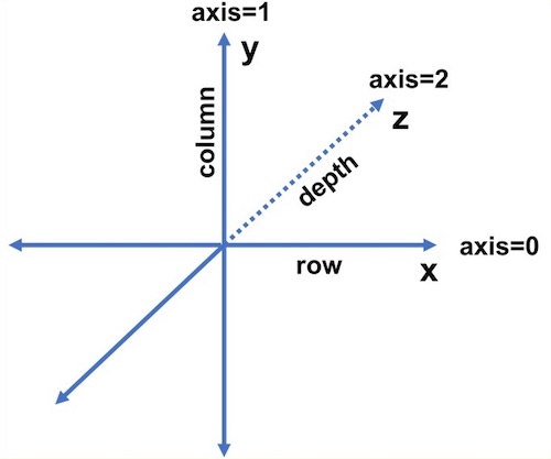
벡터는 x 축만을 갖는 자료형입니다. 1차원 배열에 해당하는 벡터의 각 요소(Element)는 그 자체가 Row입니다.
2차원 배열 형태의 행렬(matrix)은 x축의 행과 y축의 컬럼을 갖습니다. 2차원 배열 행렬은 depth가 1이라고 생각할 수 있습니다.
3차원 배열 형태의 Tensor는 행과 열을 갖고 각 컬럼은 벡터 형태를 갖습니다. 이러한 벡터를 Depth로 표현합니다.
4차원 이상의 배열은 z축의 depth 요소가 스칼라가 아니라 벡터 이상의 자료형을 갖는 것을 의미합니다. 이러한 방식으로 데이터의 Dimension(차원)은 끝없이 확장될 수 있습니다.
axis = 0 기준 row 기준 합
axis = 1 기준 column 기준 합
누락된 데이터는 NaN으로 표시
누락된 데이터를 버리는 방법
df2.dropna(how='any')
누락된 데이터를 채우는 방법
df2.fillna(value=5)
누락된 데이터인지 확인하는 방법
pandas.isna(df2)
통계 값
df2.mean()
다른 축에서 동일한 작업
df2.mean(1)
문자열 병합
concat
그룹화
groupby('A') column을 기준으로 group화
'개발' 카테고리의 다른 글
AWS EC2 환경에 nginx를 설치해 배포하는 방법. (0) 2020.10.21 [Linux] Ununtu에서 MariaDB 설치 하기 (0) 2020.10.21 https 적용하기 (0) 2020.08.12 mysql errno :150 ?~? (0) 2020.08.02 Vue 에서 is not Defined 가 뜬다면? (0) 2020.07.25